Time Series Analysis of the US Swaps Markets

I earned my Masters degree in Statistics from Columbia University in 2008. At that time in my life I was embarking on a career on Wall Street in the foreign exchange and rates markets. I wanted to spend time investigating these markets and explore some of the statistical methods I found most interesting. My masters thesis project attempted to determine appropriate models to predict long term swap rates.

Download my thesis paper here. (Give it a moment, it's a big file!)

Project Abstract

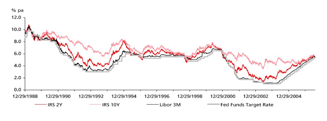
The project attempted to determine appropriate models to predict long term swap rates. ‘Long term’ was defined to be greater than five years and ‘short term’ was defined to be less than or equal to five years. The term structure of interest rates was used in order to determine a relationship between the front end and the back end of the swaps curve. That is, short term swap rates were used as explanatory variables to determine long term rates. An additional set of macro-economic exploratory variables was also used as exogenous variables to predict long term rates. The exogenous variables were: the Federal Reserve effective rate, constant maturity US treasury rates, and US Baa7 corporate bond yields. These were employed to determine to what extent, if any, these help predict long term rates.

---

R Code

#### Example R Code######## 7.6.1. 10yr Swap vs All 8 Variables ########################################### ##########ERROR FITTING PROCEDURE####### #########################################STEP 1 - PLOT LINEAR RELATIONSHIP
#plot(Tres10yr, SwapTres10yr,xlab="10 year Treasury Rate",ylab="10 year Swap Rate",main="10 Year Swaps vs Treasury Rates")
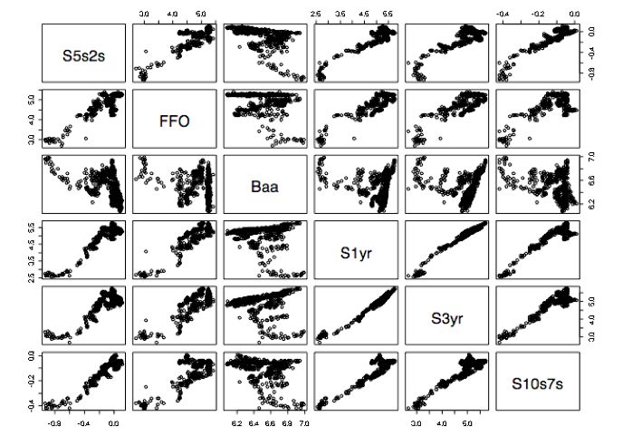
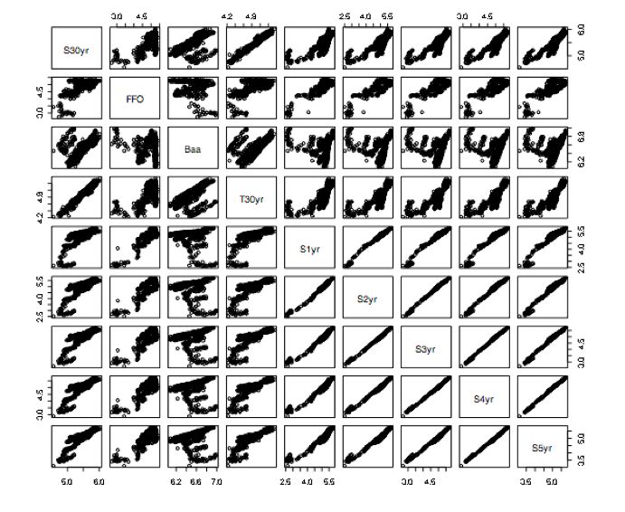
#abline(lm(SwapTres10yr ~ Tres10yr),col=2) pairs(cbind(S10yr,FFO,Baa,T10yr,S1yr,S2yr,S3yr,S4yr,S5yr))#STEP 2 - LINEAR REGRESSION/CHECK CORRELATED ERRORSlinreg<-lm(S10yr~FFO+Baa+T10yr+S1yr+S2yr+S3yr+S4yr+S5yr) linreg_res=resid(linreg)
ts.plot(linreg_res, main="Residuals", ylab="")#STEP 3 - PLOT ACF/PACFpar(mfrow=c(2,1))
acf(linreg_res, main="S10yr~FFO+Baa+T10yr+S1yr+S2yr+S3yr+S4yr+S5yr") pacf(linreg_res, main="S10yr~FFO+Baa+T10yr+S1yr+S2yr+S3yr+S4yr+S5yr")#STEP 4 - DIFF BY LAG 1/CHECK ACF/PACFres_dif<-diff(linreg_res,1) par(mfrow=c(2,1)) acf(res_dif, main="(1-B)Xt") pacf(res_dif, main="(1-B)Xt")#STEP 5 - RUN AUTOREGRESSIVE FUNCTION MINIMIZING AICfor (i in 0:4){      for(j in 0:4){        AIC=arima(res_dif,c(i,0,j),method="ML")$aic         print(c(i,j,AIC))
      }    } AR=1MA=2#STEP 6 - FIT MODEL OF RESIDUALS
#check which model gives most stable results arima_pdq<-arima0(diff(S10yr),order=c(AR,0,MA), xreg=cbind(diff(FFO),diff(Baa),diff(T10yr),diff(S1yr),diff(S2yr),diff(S3yr),diff(S4yr),diff(S5yr)),include.mean=TRUE, method="ML")
arima_pdq#STEP 7 - VALIDATE MODEL#may need to adjust order if there are NAN results - refer back to AIC output and select second lowest AIC
AR=2
MA=1arima_pdq<-arima0(diff(S10yr),order=c(AR,0,MA), xreg=cbind(diff(FFO),diff(Baa),diff(T10yr),diff(S1yr),diff(S2yr),diff(S3yr),diff(S4yr),di ff(S5yr)),include.mean=TRUE, method="ML")
arima_pdq#check that all beta estimates are significant - ellimiate those that are not based on 2*SE test
arima_pdq<-arima0(diff(S10yr),order=c(AR,0,MA), xreg=cbind(diff(Baa),diff(S2yr),diff(S3yr),diff(S4yr),diff(S5yr)),include.mean=TRUE, method="ML")arima_pdq#STEP 8 - RESIDUALS OF ARIMA MODEL - CHECK ACFresid_arima<-arima0(diff(S10yr),order=c(AR,0,MA), xreg=cbind(diff(T10yr),diff(S2yr),diff(S3yr),diff(S4yr),diff(S5yr)),include.mean=TRUE, method="ML")$resid
par(mfrow=c(2,1))
acf(resid_arima)
pacf(resid_arima)#STEP 9 - CHECK CONSTANT VARIANCEpar(mfrow=c(2,1))
ts.plot(resid_arima,main="Residuals of ARIMA(2,0,1)",ylab="") acf(resid_arima^2,main="Squared Residuals")#STEP 10 - FIT GARCH MODEL IF VARIANCE NOT CONSTANTgarch_pq<-garch(resid_arima,order=c(1,1)) garch_pq
summary(garch_pq)#STEP 11 - PLOT VARIANCEsigma.t<--garch(resid_arima,order=c(1,1))$fitted.values[,2] par(mfrow=c(2,1))
ts.plot(resid_arima, main="Residuals of ARIMA(2,0,1)", ylab="") ts.plot(sigma.t,main="Sigma-Squared of GARCH(1,1)",ylab="")########DIAGNOSTICS########
#Checking daiagnostics of the ARIMA model tsdiag(arima_pdq)#Checking normailty - maximizing the Gaussian liklihood
# if the residuals are normal then the L(phi, theta, beta) is a good fit par(mfrow=c(1,2))
hist(resid_arima)
qqnorm(resid_arima)
qqline(resid_arima)
shapiro.test(resid_arima)#Checking that the residuals of fitted model are ~ WN(0,sigma^2)par(mfrow=c(3,1))
ts.plot(resid_arima, main="Residuals of ARIMA(2,0,3)", ylab="") ts.plot(rnorm(2000),ylab="",main="White Noise") ts.plot(garch_pq$resid,main="Residuals of GARCH(1,1)")adf.test(resid_arima) pp.test(resid_arima)prod=predict(fit,n.ahead=20) ts.plot(linreg_res[1600:1645],xlim=c(0,70),ylim=c(0,.5)) abline(v=50,lty="dotted") lines(prod$pred,col="red",type="o") u=prod$pred+2*prod$se
d=prod$pred-2*prod$se
lines(u,col="blue",lty="dashed") lines(d,col="blue",lty="dashed")###For GARCH models:
###GARCH(0,1) MODEL SATISFIES THE BOX LJUNG TESTpar(mfrow=c(1,2))hist(garch_pq$residuals,main="Histogram of GARCH Residuals",xlab="Garch Residuals") qqnorm(garch_pq$residuals)
qqline(garch_pq$residuals)
summary(garch_pq)#Checking that the residuals of fitted model are ~ WN(0,sigma^2)par(mfrow=c(2,1)) ts.plot(rnorm(500),ylab="",main="White Noise") ts.plot(garch_pq$resid,main="Residuals of GARCH(1,1)")#GARCH PREDICTIONS - looking at sumer of 2008
#(PG 287 SHUMWAY)
u=predict(garch(resid_arima,order=c(0,1))) plot(360:545,resid_arima[360:545],type="l",main="Garch Predictions during Credit Crunch (Q4 '07 - Q1 '08)",xlab="",ylab="ARIMA Residuals")lines(u[,1],col="blue",lty="dashed") lines(u[,2],col="blue",lty="dashed")########## END ###################################